Creating paintings from wind patterns

Recently, I’ve been intrigued by the art of drip painting. You’ve probably come across Jackson Pollock’s beautiful canvases and as a fun experiment I tried to recreate them digitally with some Computer Vision. For this particular example, I used data from a DIY wind-sock to drive the pattern. I think its quite interesting to look at the resulting images since they are each unique and reflect the particular weather and location conditions from which they were created.

Getting started

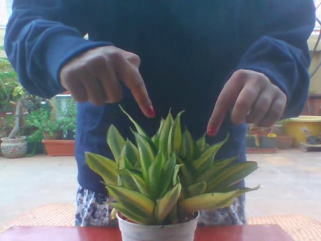
To create a windsock, I taped a circle cut out of some red paper to a length of wool. The paper does need to be heavyweight, or it flutters about quite uselessly and fails to move in a meaningful way. The wool was then tied to a long stick and held at an arms length and the red marker filmed from above.

The reason for using a red marker is because a very intense red isn’t commonly present in many natural scenes – so its quite easy to extract it out of an image. I filmed the video in my terrace and since the tile was a grey tone, it wasn’t too much trouble isolating the red.

Processing the video

Extracting the red marker

First I converted the frame to HSV colorspace. This makes it easy to locate the red tones irrespective of lighting conditions.
Then using cv2.inRange() I create a mask . If youd like to learn more about this- I highly recommend reading this blog post

frame1 = cv2.resize(frame1, (568,320)) #resize the frame to see it better
 out=np.full_like(frame1,[0,0,0])
 hsv = cv2.cvtColor(frame1,cv2.COLOR_BGR2HSV)
 lower_red = np.array([0,120,70]) #declare an upper and lower bound for the hue red 
 upper_red = np.array([10,255,255])
 mask1 = cv2.inRange(hsv, lower_red, upper_red)
 lower_red = np.array([170,120,70]) # the values for red are present next to blue as well as next to yellow 
 upper_red = np.array([180,255,255])
 mask2 = cv2.inRange(hsv,lower_red,upper_red)
 mask1 = mask1+mask2
 res = cv2.bitwise_and(frame1,frame1, mask= mask1)

Calculating the Dense Optical Flow

Im using cv2.calcOpticalFlowFarneback estimate the dense pixel motion of my marker. This returns the magnitude as well as the direction of movement of each pixel.

Setting up variables

Coordinates

Create a contour around the processed marker and calculate its center of mass. This serves as a coordinate for setting down a circle to look like a drop of paint.
I append all the coordinates to a list and handle the painting later.

Direction

Create an ROI around the marker and average the hues within this box to get an estimate of the direction. Similar to the process above, I append this to a list

Magnitude

Calculate the average lightness within the ROI to get an estimate of the magnitude and append to a list

c = max(contours, key = cv2.contourArea)
M = cv2.moments(c)
cX = int(M["m10"] / M["m00"])
cY = int(M["m01"] / M["m00"])
x,y,w,h = cv2.boundingRect(c)     
roi=hsv[y:y+h,x:x+w ]     
roi2=out[y:y+h,x:x+w ]     
roi2= cv2.cvtColor(roi2,cv2.COLOR_BGR2HSV)     
vals=np.reshape(roi,(-1,3))     
vals2=np.reshape(roi2,(-1,3))     
flat_vals=np.average(vals,axis=0)     
flat_vals2=np.average(vals2,axis=0)     
line=int(flat_vals[2]/35)+1     
hues_detected=flat_vals[0]     
hue_list.append(hues_detected)     
coords.append([cX,cY])    
movements.append(flat_vals[2])

Painting

Calculating abrupt changes in direction

After watching a few drip painting videos online, I noticed that a change in direction would be pronounced using a larger splatter. So I plotted the list of hues to take a better look at the changes in direction and found the peaks using scipy.signal.find_peaks to calculate the points at which the direction changes.

Painting!

Once you find get the information from the video, the possibilities are endless. For this particular example, I set a matrix to be white by filling it with [255,255,255] and created a black circle on top for each frame of my original video. I varied the size of the circles according to the magnitude variable and added some lines between a couple of the smaller circles for it to resemble a drip painting. In the future, I look forward to experimenting with more colors and effects to create interesting pictures.

Get the code

To try out the code,you can find a link to the jupyter notebook here. I hope you found this article interesting and I look forward to seeing your creations.

Extracting video frames corresponding to an audio signal

It’s no secret that data collection is one of the most important steps in creating an effective deep learning model. An easier way to obtain a lot of image data of a subject is to use frames from a video. Since a single second of video can ideally have 24 frames or more, it’s a pretty practical way to create relevant datasets. 

Of course, that’s the easy part. The real challenge lies with labeling all of this data.

Last weekend, I wanted to create a binary classifier using a CNN that would classify whether I touch the leaves of a plant or not. The dataset for this task would be images where I touch the leaves of a plant and images where I am not touching the leaves of the plant. As a method of collecting some data, I decided to record a video of alternating between touching the plant and not touching the plant with the times I touch the plant pronounced by a loud gong sound in the background operated by my trusty assistant.

The idea here is really simple : find the frames that correspond to the loud sound in the background 

Preparing the data

Firstly, it’s a good idea to separate the audio from the video and save it as a different file. Additionally, I converted the audio signal from stereo to mono using audacity so that the resulting signal only had one channel. 

I’m reading in the data using python’s wave module, and then converting to a numpy array so that I can find the maximum value of the signal. For my example, the maximum is 32767. However, since I know that some of the gong sounds were softer than the others, so I’m going to find the peaks in the signal that correspond to a number greater than 30000. This is definitely an arbitrary choice, and playing with this value would yield different results.

Finding the coinciding frames

Comparing the framerate of my audio and video sample, I notice that the rate of my audio is 44100 frames per second, while my video consists of 30 frames per second. With some simple math, its easy to see that this means each frame of video corresponds to about 1470 frames of audio. The scipy find_peaks function conveniently returns the position of the array which contains the peak. Dividing this position by 1470 gives me the video frame that contains the peak that I want.

 

Extracting the frames

I’m using opencv to cycle through the video frames and save them to specific folders. For now I’m using the first portion of the video as my training dataset and the latter portions for validation and testing.

plant_touch/datastr/test/touch/6313.jpg

/home/skb/penv/plant_touch/datastr/test/notouch/6276.jpg

This method isn’t entirely perfect, owing to multiple factors such as human error ( the gong may not always sound at the right time) , ambient noise as well as choosing an arbitrary cut-off point, but its a really easy way to quickly get labelled data and although I’ve demonstrated this technique with a really specific use case, I hope you find it useful in your own projects.

If you’d like to take a look at the code, you can find it here

Please feel free to leave any feedback/ suggestions and I’ll get back to you as soon as I can

Transfer Learning with Tensor Flow using the CIFAR-10 dataset and Google Compute Engine

Part 1: Running a Jupyter notebook on Google Compute Engine

The first step is to get a Jupyter notebook up and running. Of course it isn’t necessary to use Jupyter to run all the code but I have a personal preference for the workflow it offers. There were two ways that I was able to achieve this. The first-to create a new instance and download all the libraries I needed.

This is a time consuming process, as sometimes there are compatibility issues when using a different version of the library. I experienced this when trying to use tensorflow after an anaconda installation. The workaround was to create a separate anaconda environment and install tensorflow there.

To run the Jupyter notebook, I created a reserved a static IP address, changed the Jupyter configuration files and ran the notebook on the server. However note that this makes the notebook publicly accessible. While, Jupyter does provide a layer of security by requiring web token authorization, it’s not a good practice to do this.

The second way I tried this was to create a VM instance from a machine image. This was a much faster way to get up and running. It involved first installing the and authenticating the Google CLI on my local machine, and then creating an instance from the command line. There’s a really handy tutorial here that helped me get up and running pretty quickly. I used a ‘tf-latest-cpu’ image on an ‘h1-highmem-8’ which is an 8 core cpu with 200 GB memory space. I’m also using a preemptible instance which cuts costs but the downside is that the machine only runs for 24 hours and can be interrupted at any time. However, Google does state that the ‘preemption rates for smaller machine types with less than 32 cores are also historically lower than for larger machine types’ and I didn’t intend on running the machine for longer than 24 hours anyway.

Once the instance has been created, the next step is to connect to it via SSH. This can be achieved both through the User Interface or through the command line. Note that you’re only connected to the instance as long as the SSH connection persists.

connecting through command line

connecting from the browser

Now all I have to do is navigate to http://localhost:8080/tree?

Part 2: What is transfer learning ?

Despite how accessible computation power to train neural networks has become today – a significant caveat still remains: obtaining enough training data for the model to learn from and produce satisfactory results.

Transfer learning is a process by which a pretrained model is reused for a similar classification task. For example, if we had a network already trained to classify types of buses, then there’s a good chance we can reuse this to classify types of trucks. The process commonly involves freezing a few of the lower layers, which means that we preserve the previously learned parameters and as an added advantage reduces the time required for training our entire model.

Many popular model architectures as well as their pre-trained weights are available in the TensorFlow keras applications module.

For the following task I’ve experimented with two model architectures – VGG16 and ResNet50.

Part 3: CIFAR10 with ResNet50

The CIFAR-10 dataset available here is a dataset of 32 x 32 colour images belonging to 10 classes. It can be directly downloaded via TensorFlow and is conveniently subdivided into training and testing datasets.

Additionally I created a validation dataset from a part of the training dataset. It’s important to have a validation dataset since it helps us determine whether the model has really learnt relevant features or simply memorized the training dataset.I also encoded the labels into a one-hot format to use with softmax later.

splitting the data

converting labels to one-hot format

using the summary() method to view the layers in a resnet50 architecture

Next, I instantiated a ResNet50 architecture with pretrained weights from the image net challenge ( here’s the documentation). Since the default input shape was 224 x 224, I decided to resize my images, before feeding it to the model. Initially, I intended to use skimage.resize, however resizing 50,000 images to 224 x 224 ended up taking up too much space and I found an easier approach as mentioned in this super useful answer and that was to create a lambda layer.

A lambda layer basically performs custom operations on the data. It can be added to the pipeline when creating a Sequential model. So I created a lambda layer and resized my images with tf.image.resize.

Since the training process was going to take quite a while, it’s also useful to save the model between epochs so as to not have to train from the beginning if the process is interrupted. Here’s a useful medium article illustrating how to do that.

On top of the lambda layer, I added my base model (ResNet50), an averaging layer, a dense layer with 10 units( since CIFAR-10 has 10 classes) and a softmax layer to predict the final output. In this example I’m not going to train the base model at all.

All that’s left is to compile the model and fit the training dataset. I’m going to run the model for 10 epochs with a batch size of 64.

After the 10th epoch, I notice that while the training accuracy has increased, the validation accuracy has converged to around 65 % . This is a sign of overfitting.

Part 4: CIFAR10 with VGG16

For this example, I followed the same steps as the previous example, but instead of increasing the size of my image, I changed the shape of the input layer of the network. As a base model, I’m using VGG16. However this time, I’m going to train the entire network and see what kind of results I get.

The VGG16 architecture

I’m also using a technique here called learning rate annealing. This basically reduces the learning rate by a factor if certain conditions are met. Since a high learning rate is good for finding the minima faster, its often good to start with a higher learning rate and reduce it if the validation accuracy does not change

Here I’m going to reduce the learning rate by a factor of 0.01 if the validation accuracy doesn’t change after three epochs.

However as you can see, the model seems to be overfit once more.

Further improvements:

Since, the results of the above two examples weren’t very good; in the next post I’m going to try to examine the reasons behind this and how to overcome them. I’m also going to try to create a binary classifier with a dataset from images I collect myself and see what happens.

Sunglass filter with MTCNN

If you’ve ever used Snapchat or Instagram, you’ve probably come across the popular sunglass filters, that superimpose a pair of sunglasses on your face

The way this works is quite straightforward- First facial keypoints are obtained, and then the new image is overlaid on top of the camera input, corresponding to those keypoints.

In this post, I’m going to try an recreate that using OpenCV with Python. Of course, this is just a simple version to explore the various possibilities of image recognition.

To obtain the keypoints, ideally we’d want to train our own classifier. However I’m going to use mtcnn, a pretrained classifier which works pretty well and returns as keypoints- the position of eyes, nose and mouth.

For the sunglasses, I cropped this free stock photo, and saved it as a png since I wanted to work with the transparent background. However, there’s an alternative way to extract the image, if you don’t have a png image. You can find it on the OpenCV documentation here

To overlay the image, I found this really useful answer here which is a great explanation of how to add a transparent image to an image with three channels.

Next we want to detect the face using mtcnn and extract the position of the eyes. This should give a result as follows:

mtcnn returns a list of json objects. You can find “nose” under the “keypoints” key:

I also want to change the size of the sunglasses depending on the width of the bounding box returned. Since I only have the keypoints corresponding to the eyes, these dimensions are just a matter of preference:

The final part is to select an ROI [ Region Of Interest]. I used the height and width of the sunglasses to select the region around the eyes, and superimposed the resized sunglasses on top.

Get the Code:

You can find the full code for this project on my github.

Improvements:

Of course, this does not look the same as the actual sunglass filters you find on Instagram. Part of this is due to the lack of feature points, which adds a bit of guesswork to fitting the sunglasses on the face.

Another improvement could be adding images in different orientations, for the application to be able to handle changes in perspective, rotation, etc.

Optical flow with the Lucas-Kanade algorithm

Optical flow is the apparent motion of pixels between consecutive frames of a video. Ideally we’d like to find a vector that describes this motion or a displacement vector that indicates the relative position of a particular pixel in another frame

Trying to do this for every pixel in an image is known as dense optical flow. However this is can be quite computation heavy, so we turn our attention to a different class of algorithms called sparse optical flow algorithms, that track only a specific number of points in the image.

The Lucas-Kanade algorithm

The Lucas-Kanade algorithm is popular in problems concerning sparse optical flow. This is because it requires small windows of local interest.

Optical Flow makes two assumptions:

1- Consistent Brightness:
A pixel’s brightness remains the same as it moves from frame to frame

2-Temporal persistence
The motion of an image is coherent. This means that the motion of our window of interest changes relatively slowly from one frame to the next

Let’s first look at the motion in one dimension:

Mathematically, the equation for constant brightness can be expressed as:

I(x(t),t)=I(x(t+dt),t+dt)

Since the brightness of a pixel is considered to be constant over time, the intensity of a pixel at time t is equal to the intensity of a pixel at time t+dt . Of course, we can also conclude that the partial derivative is:

∂f(x) /  ∂t = 0

where f(x) ≡ I (x(t),t)

For our second assumption, we can note that the motion is very small from frame to frame. So we can say that the change between frames is differentially small. Now since we’re only looking at one dimension

We know that the function describing brightness f(x,t) is dependent on t, I(x(t),t), so we can substitute this definition and apply the chain rule, to obtain:

I_x.v + I_t = 0

I_x here is the spatial derivative across the first image while I_t is the temporal derivative.

We need to find the value of v

By switching the terms around we get :

v= -I_t/I_x

However the assumptions that we made at the beginning, i.e. the assumption that the brightness is stable and the motion of the pixel from frame to frame is small is not always true. However, if we are reasonably close to obtaining a solution for v, we can iterate toward an answer.

We can do this by keeping our spatial derivative same and changing the temporal derivative. Eventually the iterations should converge.

Lets try this with two dimensions:

I(x,y,t)= I(x + Δx,y+Δy,t+Δt)

We can reduce this expression to:

[u(x,y,t)∂I(x,y,t)/∂x]+[v(x,y,t)∂I(x,y,t)/∂y ]+[∂I(x.y,t)/∂t]=0

Here, I’m calling the velocity component in x direction u and the velocity in the y direction v.

However, now we have two variables u and v but only one equation. This equation is underconstrained!

To get around this, a third assumption is made:

3. Surrounding pixels to the pixel of interest have a similar motion to the pixel.

This implies that we can use the surrounding pixels, ie. get a patch of pixels, to set up more equations to solve for the two unkn0wns:

A little bit of matrix math, and we obtain the solution as:

where our first matrix is represented by A and the other as matrix b.

From this equation, we see that the A^TA is invertible when it has two large eigenvectors. This occurs if the point we use has gradients in two directions. This property is best seen in corners which is why it makes sense that the corners are good features to track!

Lucas-Kanade pyramid

Earlier we’d assumed that the motion from frame to frame was small. Unfortunately, in the real world, this is rarely the case where in videos captured by a camera, noncoherent and large motions are quite commonplace.

As a workaround, we can track the motion in a large space with an image pyramid and then use our assumed velocity to work down the image pyramid until we arrive at the original image size. That is, we solve for the top layer and use the solution as an estimate for the next level and so on.

Implications:

From the derivation, we can see that the Lucas-Kanade algorithm isn’t going to work well on images with smooth shading. The more texture an image has, the better it is for tracking. It’s also quite difficult to track edges , since edges have large eigenvectors in one direction only.

Further reading:

I hope this serves as a brief look under the hood of the workings of the Lucas-Kanade algorithm. For a more insightful view -check out these resources:

• Learning OpenCV3 by Gary Bradski – written by the creator of OpenCV, this book is an intensive look into Computer Vision
• Implementing Optical flow with OpenCV – From the OpenCV docs
• Harris-Shi-Tomasi corner detection